Sharing Data across Worksheets and Workbooks

Moving and Copying Data between Worksheets

You can move and copy data between worksheets just as you do within a single worksheet. Instead of specifying the paste destination in the source worksheet, you specify the paste location in a second worksheet, called the destination worksheet, which can be in the same or another workbook. When you move or copy cells or ranges that contain formulas and functions, you must take into account whether or not they employ relative or absolute references.

For Instructor-led Excel training in Los Angeles call us on 888.815.0604.

Method

To move data between worksheets:

Ribbon method

1. In the source worksheet, select the data you want to move.
2. On the Home tab, click the Cut button in the Clipboard group.
3. In the destination worksheet, select the desired location for the data.
4. On the Home tab, click the Paste button OR
5. Press Enter

Mouse method

1. Tile the source and destination worksheet windows.
2. In the source worksheet, select the data you want to move.
3. Drag the data to the desired location in the destination worksheet.
4. To copy data between worksheets:

Ribbon method

1. In the source worksheet, select the data you want to copy.
2. On the Home tab, click the Copy button.
3. In the destination worksheet, select the desired location for the data.
4. On the Home tab, click the Paste button OR
5. Press Enter

Mouse method

1. Tile the source and destination worksheet windows.
2. In the source worksheet, select the data you want to copy.
3. Press and hold Ctrl.
4. Drag the data to the desired location in the destination worksheet.
5. Release Ctrl

Exercise

In the following exercise, you will move and copy data between worksheets.

1. In the Advertising Workbook choose the Mass Mailing 2000 worksheet, select cells B5:B9
2. On the Home tab, click the Copy button. [A moving border appears around the selected range].
3. Select the SUMMARY worksheet, and then select cell B5.
4. Press Enter. [The range is pasted into the SUMMARY worksheet].
5. From the Window group located in the View tab, choose New Window. [A copy of the Advertising workbook window appears].
6. Tile the SUMMARY and Mass Mailing 2001 worksheet windows.
7. In the Mass Mailing 2001 worksheet window, select the range B5:B9.
8. Drag the selected source data to the SUMMARY worksheet window, to the range C5:C9. [As you drag, the right worksheet window becomes active and an outline appears the size of the selected data. Then, the data is moved to the new location].
9. Press and hold Ctrl.
10. In the SUMMARY worksheet window, drag the selected data back to the Mass Mailing 2001 worksheet window, to the range B5:B9. [A plus sign is added to the mouse pointer when positioned over the border of the selected range. As you drag, the right worksheet window becomes active and an outline the size of the selected data appears].
11. Release Ctrl. [The 2001 data appears in both worksheet windows].
12. In the left worksheet window, select the Mass Mailing 2002 worksheet, and then select cells B5:B9.
13. On the Home tab (clipboard group), click the Cut button. [A moving border appears around the selected range].
14. In the right worksheet window, in the SUMMARY worksheet, select cell D5.
15. On the Home tab (clipboard group), click the Paste button. [The data is moved to the new location and is too long for the cell width].
16. Click the Undo button. [The data is returned to the source worksheet. The selected range has a moving border around it].
17. Press Esc. [The moving border disappears].
18. Close the left worksheet window.
19. Maximize the remaining worksheet window.

Linking Data Between Worksheets

When you link data between worksheets, it becomes dynamic. In other words, if you change the data in the source worksheet, you automatically change the linked data in the destination worksheet. You can use linked data to create dynamic formulas and to keep your worksheets in agreement.

Linking Data with the Paste Special Command

One way to link data is to paste a copy of it in the destination worksheet using the Paste Special dialog box, shown in Figure 1-7. In this way, you ensure that both the source data and the copy are updated.

Because linking involves multiple worksheets, Excel uses 3-D references. A 3-D reference consists of the name of the source worksheet in single quotes, followed by an exclamation mark and the cell reference, range reference, or range name. For example, ‘Mass Mailing 2002’!B5 refers to cell B5 in the Mass Mailing 2002 worksheet. You will see a 3-D reference in the Formula bar when you select a cell containing linked data.

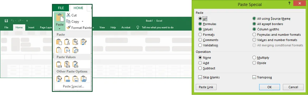
Figure 1-7: The Pate Special Options from Paste buttons and Paste Speical Dialog Box

Method

To link data between worksheets:

1. In the source worksheet, select the data to be linked.
2. On the Home tab (clipboard group), click the Copy button.
3. In the destination worksheet, select the location for the linked data.
4. On the Home tab (clipboard group), choose Paste > Paste Special.
5. In the Paste Special dialog box, choose Paste Link.

Exercise

In the following exercise, you will link data between worksheets.

1. In the Mass Mailing 2002 worksheet, select cells B5:B9.
2. On the Home tab (clipboard group), click the Copy button. [A moving border appears around the selected range].
3. In the SUMMARY worksheet, select cell D5.
4. From the Clipboard group on the Home tab, click the drop down arrow, choose Paste Special. [The Paste Special dialog box appears].
5. Choose Paste Link. [The dialog box closes, the data is pasted, and the formula bar shows a 3-D reference].
6. If necessary, widen the column to view all data.
7. Select the Mass Mailing 2002 worksheet. [The moving border is still around the selected range].
8. Press Esc. [The moving border disappears].
9. Edit the contents of cell B5 to read 1,186,521.
10. Check the SUMMARY worksheet to see any changes. [The data in cell D5 is updated].