Creating multiple views in Excel

Creating Multiple Views

In many cases, you might find it helpful to work with different sections of your worksheet at the same time. You might, for example, want to keep the labels in row 4 visible while you scroll down to look at information located in row 35. You do this by applying either split bars or freezing panes.

For live face-to-face Excel training in Los Angeles call us on 888.815.0604.

Applying Split Bars

When you apply split bars to a worksheet, Excel creates identical copies of the worksheet side by side. Split bars are illustrated in Figure 1-3. If you apply either a horizontal or vertical split bar, you can scroll within one pane while the other pane remains stationary. If you apply both horizontal and vertical split bars, in which four panes are created, only two panes remain stationary when you scroll within one pane. For example, if you horizontally scroll in the upper right pane, you simultaneously scroll through the lower right pane while the two left panes remain stationary.

Although the Split command can be accessed from the Windows group on the View tab, you can also manipulate split bars with the mouse using the split boxes shown in Figure 1-4.

You can move between the different panes by simply clicking the pane in which you want to work. Because each pane is a view of the same worksheet, a change in one pane means a change to the worksheet.

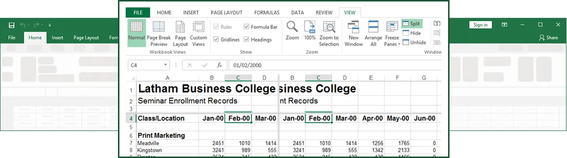
Figure 1-3: Worsheet Split Bars

Method

To apply horizontal and vertical split bars:

1. Click the cell to the right of the location for a vertical split and below the location for a horizontal split.
2. From the Windows group on the View tab, choose Split.

To apply a horizontal or vertical split bar:

1. Position the mouse pointer over the horizontal or vertical split box.
2. When the mouse pointer changes to a split pointer, drag the split box down or left to the desired location.

To remove a split bar:

1. Double-click any part of the split bar that divides the panes.

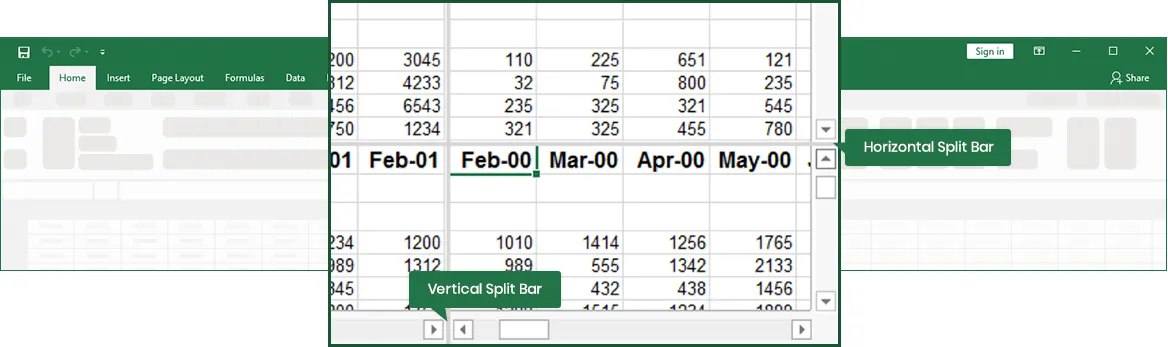
Figure 1-4: The Split Boxes

Exercise

In the following exercise, you will apply split bars.

1. Select the Enrollment by Seminar worksheet.
2. Select cell B5.
3. From the Windows group on the View tab, choose Split. [The worksheet is split into four panes].
4. Double-click any part of the split bar that divides the panes. [The split bars are removed].
5. Position the mouse pointer over the vertical split box. [The mouse pointer changes to a split pointer].
6. Drag the vertical adjustment to the right of column B. [As you drag, an outline of the split bar appears. Then the window is split into two panes. Because cell B5 was selected, the left pane is now selected].
7. Use the Name box to select cell V7. [Cell V7 is visible in the left pane. The right pane does not change].
8. Drag the vertical split bar to the left edge of the worksheet window. [The split bar is removed].

Freezing Panes

Another way to divide your worksheet into panes is by freezing sections of the worksheet. Freezing panes is useful when you are working with large tables because you can hold horizontal and vertical labels stationary while you move through the data.

Method

To freeze panes of data:

1. Select the cell below and to the right of the location for the frozen panes.
2. From the Window menu, choose Freeze Panes.
3. Note: If the cell you select is in column A or in row 1, choosing Freeze Panes will result in two panes instead of four.

To unfreeze panes of data:

1. From the Window menu, choose Unfreeze Panes.
2. Note: When you freeze panes, the Freeze Panes option changes to Unfreeze Panes so that you can unlock frozen rows or columns.

Exercise

In the following exercise, you will freeze and unfreeze worksheet panes.

1. Select cell B13.
2. From the Window menu, choose Freeze Panes. [The worksheet is divided into four panes. The panes are separated by thin, dark lines].
3. Press Right Arrow until you can see the Dec-95 column. [The labels in column A remain stationary as you scroll to the right].
4. Press Page Down twice. [Rows 1 through 12 remain stationary as you scroll].
5. From the Window menu, choose Unfreeze Panes. [The worksheet is restored to a single pane, and the thin, dark lines are removed].

Viewing and Arranging Multiple Worksheet Windows

Often, it is useful to view more than one worksheet at a time. You can arrange worksheets on your screen so that you can view them simultaneously. Once you have more than one copy of your worksheet window open, you can select different worksheets to view from each worksheet window, and then arrange the windows to best suit your needs. For example, Figure 1-5 displays four worksheets from the same workbook at once. Once you have arranged the worksheet windows, you can move between different windows simply by clicking the window in which you want to work. It takes one click to activate a window and another click to select anything in that window.

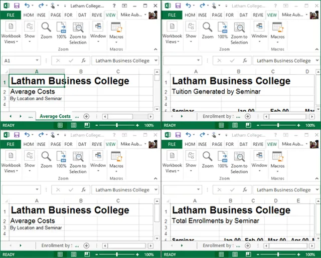
Figure 1-5: Tiled Worksheets

The Arrange Windows dialog box provides options to let you set up your data on the screen. These options are summarized in Table 1-2.

Option	Function
Tiled	Arranges windows so that each fills an equal portion of the work area.
Horizontal	Arranges windows one below the other.
Vertical	Arranges windows next to each other.
Cascade	Stacks the windows, offset vertically with the title bar of each window showing.
Windows of active workbook	Provides views of only the currently active workbook when other workbooks are open.

Table 1-2 : The Arrange Windows Dialog Box Options

Method

To view and arrange multiple worksheet windows:

1. Select the Book/sheet you’d like to view full-size. From the Window group on the View tab, choose New Window.
2. This opens a copy in Read Only mode.
3. Repeat steps 1 and 2 for each worksheet you want to view. Closing copies and returning as required.
4. In the Window group, choose Arrange All.
5. In the Arrange Windows dialog box, in the Arrange area, select the desired option.
6. If necessary, select the Windows of active workbook check box.
7. Choose OK.

Exercise

In the following exercise, you will view and arrange multiple worksheet windows.

1. From the Window group on the View tab, choose New Window. [A copy of the worksheet window appears on top of the original, and the window number is referenced in the title bar].
2. In the new window, select the Total Enrollment worksheet.
3. From the Window group, choose New Window. [Another copy of the worksheet window appears and the window number is referenced in the title bar].
4. In the new window, select the Tuition Generated worksheet.
5. From the Window group, choose New Window. [Another copy of the worksheet window appears and the window number is referenced in the title bar].
6. In the new window, select the Average Costs worksheet.
7. From the Window group, choose Arrange. [The Arrange Windows dialog box appears].
8. In the Arrange area, make sure the Tiled option button is selected.
9. Choose OK. [The worksheet windows are tiled].
10. Click anywhere in the top right worksheet window. [The second worksheet window becomes active. Scroll bars appear].
11. Close copies 2,3, and 4 of the workbook by clicking their Close buttons.
12. Maximize the remaining worksheet window. [The Enrollment by Seminar worksheet is active and fills the window].