Editing Excel Records Using the Data Form

You can edit any data that appears in an edit box in a data form. If record data appears with no edit box, then you cannot edit this data in the data form because the field contains a formula.

If you edit a record and then decide to cancel your edit, you can choose Restore. You must choose Restore before choosing New or scrolling to another record; otherwise, the Restore button will be dimmed and you will not be able to cancel your edit.

For instructor-led Microsoft Excel classes in LA call us on 888.815.0604.

Method

To edit a record using the data form:

1. In the data form, move to the record you want to edit.
2. Click the desired edit box.
3. Make the desired changes.
4. If desired, move to the next edit box in which you want to edit the data.
5. Press Enter or scroll to another record to accept the edit and keep the data form open. or
6. Choose Close.

To restore an edited record using the data form:

1. Choose Restore before pressing Enter, choosing New, scrolling to another record, or closing the data form.

Exercise

In the following exercise, you will enter column labels in a list.

1. Open the Car Comparison workbook, and, if necessary, select the Rental worksheet.
2. Open the data form for the list.
3. Scroll until the record with ID NO 33 is displayed. [The record for the Ford Festiva is displayed].
4. Click the IN edit box.
5. Change n to y. [The Restore command is active].
6. Move the data form so the record for the Ford Fiesta in the worksheet is visible . [The n in the IN column is still displayed in the worksheet].
7. Click the bottom scroll arrow repeatedly until the record with ID NO 3 is displayed. [The n changes to y in the worksheet in the In field for the Fort Fiesta as soon as you click the scroll arrow. The record for the Ford Tempo is displayed in the data form. The Restore button is dimmed and no longer active].
8. Move the data form so the record for the Ford Tempo (ID NO 3) in the worksheet is visible.
9. Click the DOORS edit box.
10. Change 4 to 2. [The 4 is still displayed in the worksheet, and the Restore button is active].
11. Choose Restore. [Excel changes the 2 back to a 4 in the Doors field for the Ford Tempo. The Restore button is dimmed and no longer active].
12. Close the data form.

Adding and Deleting Fields in a List

In addition to editing records, Excel lets you alter the list structure by adding and deleting fields. You add fields to a list by adding columns. If you add a new column, Excel automatically includes the new column within the list. You delete a field by deleting the appropriate column from the worksheet.

Method

To add a field to a list:

1. Select the column that will be to the right of the new column.
2. In the Cells group on the Home tab, click the Insert button.
3. In the appropriate cell, enter the column label.or
4. If the new column will be the last column in the list, in the appropriate cell, enter the column label.

To delete a field from a list:

1. Select the column containing the field that you want to delete.
2. In the Cells group on the Home tab, click the Delete button

Exercise

In the following exercise, you will add a field to a list, and then you will delete the added field.

1. In cell I1, enter MILES.
2. Open the data form for the list. [The new field name and edit box appear in the data form].
3. Close the data form.
4. Select column I.
5. In the Cells group on the Home tab, click the Delete button. [The MILES column is deleted].
6. Select column G.
7. In the Cells group on the Home tab, click the Insert button. [A new column is inserted to the left of the RATE column].
8. In cell G1, enter MILES.
9. Open the data form for the list. [The new field name and edit box appear in the data form].
10. Close the data form.

Finding Records in a List

A computerized list gives you the ability to quickly and easily search for information meeting any criteria that you specify. The Criteria button of the data form allows you to search for a particular record based on the information you enter in the edit boxes. You can search using a single criterion or multiple criteria. You can also search for exact matches, or, by using operators such as > or <, you can search for data in a specific range.

If no records meet all search criteria, the current record will be displayed. Because searches are not case-sensitive, you can type the criteria in uppercase or lowercase letters without affecting the results of your search.

Method

To find records in a list:

1. Open the data form.
2. Choose Criteria.
3. Select the field on which you want to base your search.
4. Type the desired operator (=, >, <, >=, <=).
5. Type the desired value.
6. Repeat steps 3 to 5 for each criterion.
7. Choose Find Next to find the next record in the list that meets the search criteria. or
8. Choose Find Prev to find the previous record in the list that meets the search criteria.

Exercise

In the following exercise, you will find records using a single criterion, and then you will find records using multiple criteria.

1. Select the Cars worksheet.
2. Open the data form for the list.
3. Choose Criteria. [Criteria appears in the upper right corner of the data form. All edit boxes are empty, the New button is dimmed, and the Clear button has replaced the Delete button].
4. Click the MAKE edit box.
5. Type Ford.
6. Choose Find Prev. [A beep indicates that there are no previous records meeting the criterion. The first record of the list is displayed].
7. Choose Find Next. [The first record meeting the criterion is displayed].
8. Continue to choose Find Next until you hear a beep indicating that you have viewed all the records meeting the criterion.
9. Choose Criteria. [Ford appears in the MAKE edit box].
10. Choose Clear. [The previous search criterion is cleared from the data form.he previous search criterion is cleared from the data form].
11. Click the MAKE edit box.
12. Type Chevy.
13. Click the DOORS edit box.
14. Type 2.
15. Choose Find Prev. [The first record meeting both criteria is displayed].
16. Continue to choose Find Prev until you hear a beep indicating that you have viewed all the previous records meeting the criteria.
17. Choose Criteria. [Chevy appears in the MAKE edit box, and 2 appears in the DOORS edit box].
18. Choose Clear. [The previous search criteria are cleared from the data form].
19. Click the RATE edit box.
20. Type >29.95.
21. Click the MAKE edit box.
22. Type Dodge.
23. Choose Find Prev. [A beep sounds immediately, indicating that no previous records meet these criteria].
24. Choose Find Next until you hear a beep indicating that you have viewed all records meeting the criteria.
25. Close the data form.

Sorting a List

To rearrange the records in your list in a specific order, you can sort the list based on the fields identified by the column labels. To sort a list, you can use a single criterion, such as the last names of the individuals or the state in which the individuals live. In a very large list, you can use multiple criteria, such as a last name and a first name.

To sort a list, you first select a cell in the list, just as you would before accessing the data form. You then specify the fields to sort by in the Sort dialog box, shown in Figure 1-11.

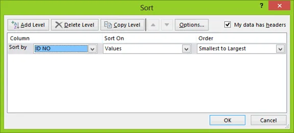
Figure 1-11: The Short Dialog Box with one Sort level created

When you sort data, Excel rearranges rows, columns, or individual cells using the column sort order that you specify, either ascending order (A-Z or 1-9) or descending order (Z-A or 9-1). If you do not specify a specific order, Excel sorts the rows in ascending order.

Microsoft Excel uses the following guidelines when sorting lists:

1. Rows with blank cells are placed at the bottom of the sorted list.
2. Hidden rows are not moved.
3. Values are sorted before text and before numbers formatted as text.
4. Numbers formatted as text are sorted before text alone.
5. The sort options are saved from the last sort done until the column labels or the sort is changed in the list.

You can add Sort ‘levels’. This constitutes ‘Then by’ sorts. Meaning multiple sort criteria, processed in the order of the sort instruction at the top of the list, descending downwards.

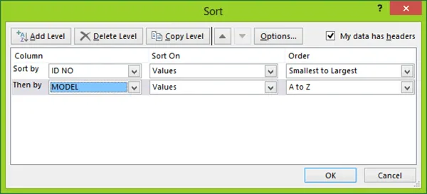
Figure 1-12: The Short Dialog Box with one Sort level created ("Sort by" plus one "Then by")

Method

To sort a list:

1. Select a cell in the list you want to sort.
2. In the Sort and Filter group on the Data tab, click the Sort button.
3. In the Sort dialog box, from the Sort by drop-down list, select the first column by which you want to sort your list.
4. Select an option in the Order section of the Sort by fields (options).
5. If desired, click the Add level button, creating the first of a ‘Then by’ list of sort instructions. Select the second list column by which you want to sort your list.
6. Select the Ascending or Descending ORDER options.
7. If desired, add another level and in the second Then by drop-down list, select the third column by which you want to sort your list.
8. Select the required Ascending or Descending options.
9. Make sure the My Data has Headers check box is checked.
10. Choose OK.

Exercise

In the following exercise, you will sort a list.

1. Select a cell in the Cars worksheet list.
2. In the Sort and Filter group on the Data tab, click the Sort button. [The Sort dialog box appears, and the list is selected].
3. From the Sort by drop-down list, select ID NO.
4. Make sure the Sort is on Values and the Order is Smallest to Largest.
5. Make sure not to add any Sort levels.
6. Make sure the My Data has Headers check box is checked, and then choose OK. [The list is sorted by ID number].
7. In the Sort and Filter group on the Data tab, click the Sort button. [The Sort dialog box appears, and the list is selected]
8. From the Sort by drop-down list, select MAKE.
9. Make sure the Sort is on Values and the Order is A-Z.
10. Add a level and in the Then by line, select MODEL as the active column.
11. Make sure the Sort is on Values and the Order is A-Z.
12. Make sure the My Data has Headers check box is checked, and then choose OK. [The list is sorted first by MAKE and then by MODEL].
13. Save the workbook.