Filtering a list in Excel
Filtering can give you more control over your list, particularly if your list contains a large number of records. For example, suppose you operate a small grocery store and have a master inventory of all the items in the store. Your list would include everything from dairy products to fresh vegetables to cookies. What if you suddenly needed to know how many types of cheese were on the shelf? You could scroll through the entire list, counting the cheeses as you go, but it would make more sense to filter the list so that it displays only dairy products, or better yet, only cheeses.
Filtering a list lets you find and work with a subset of the data in your list by displaying only the records that contain a certain value or meet specific criteria. The remaining records are hidden from view until you instruct Excel to display them again. You can then copy this filtered list to another location without disturbing the primary source list.
Using AutoFilter
Choosing AutoFilter from the Sort and Filter group on the Home tab applies drop-down arrows directly to column labels in your list, as illustrated in Figure 1-13. You then select a specific value from one of the drop-down lists to display all records in your list containing that value. For example, you can select Ford from the MAKE column drop-down list to display only those records for Ford cars.
For instructor-led Microsoft Excel classes in Los Angeles call us on 888.815.0604.
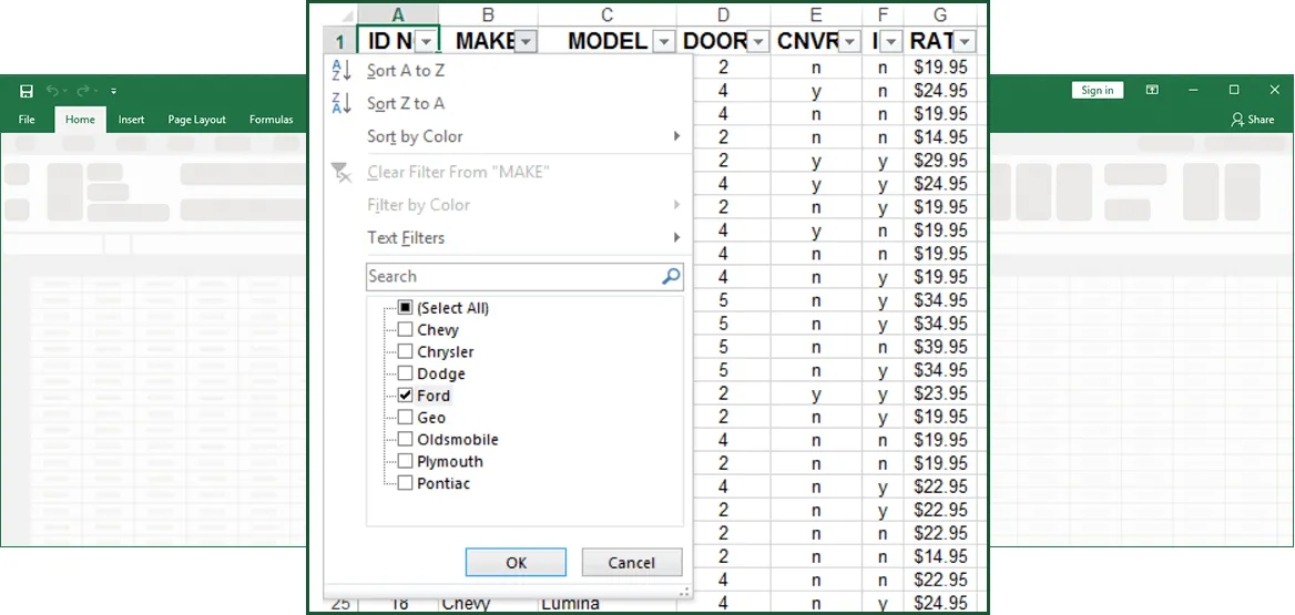
Figure 1-13: Auto Filter Dropdown Arrows
Method
To filter a list using AutoFilter:
- Select a cell in the list you want to filter.
- In the Sort and Filter group on the Home tab, click the Filter button.
- In the desired column heading cell, from the AutoFilter drop-down list, select the desired items by selecting/deselecting.
- Repeat step 3 to filter the list by other columns.
To deactivate AutoFilter:
- In the Sort and Filter group on the Home tab, click the lit-up Filter button.
Exercise
In the following exercise, you will filter a list.
- Make sure a cell in the Cars worksheet list is selected.
- In the Sort and Filter group on the Home tab, click the Filter button. [The Filter is switched on and the Filter button is illuminated].
- Look at the titles of the list of data. [The AutoFilter drop-down arrows appear in the headings of the list].
- From the MAKE AutoFilter drop-down list, deselect Select All and click to select Ford. [Only records that contain Ford in the Make column are visible. All other records are hidden. The MAKE AutoFilter drop-down arrow and the row headings of the visible records are blue].
- From the DOORS AutoFilter drop-down list, deselect Select All and click to select 2. [Only Ford cars with 2 doors are visible. The DOORS AutoFilter drop-down arrow is also blue].
- From the MAKE AutoFilter drop-down list, select only Chevy. [Only Chevy cars with 2 doors are visible].
- In the Sort and Filter group on the Home tab, click the Filter button. [The Filter dropdown arrows disappear].
- Save and close the workbook.
Custom AutoFilter Criteria
The Custom AutoFilter command lets you customize the criteria, by which you filter your list, using one or two comparison criteria. This is similar to searching for specific records using the data form; however, all your results are displayed in the worksheet, as opposed to scrolling through the records. Another advantage of using a custom AutoFilter is that you can display records that meet one criterion or the other.
For example, you can create a list of all employees with salaries greater than $40,000 and less than $55,000 or a list of all employees with salaries greater than $60,000 or less than $20,000. You specify custom criteria using comparison operators in text form, such as equals, in the Custom AutoFilter dialog box, shown in Figure 1-14. Note that in Figure 1-15 the Custom AutoFilter is using text operators as criteria as opposed to numeric ones. The Custom AutoFilter options are context sensitive and the criteria options will reflect the data in the list column being filtered.
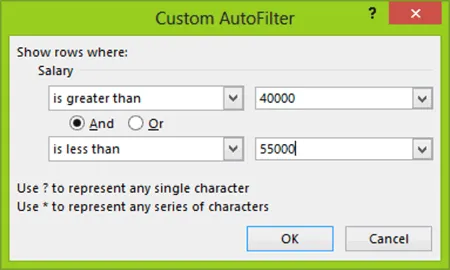
Figure 1-14: The Custom AutoFilter Dialog Box (numeric criteria)
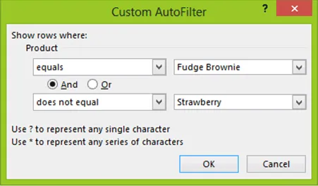
Figure 1-15: The Custom AutoFilter Dialog Box (Text criteria)
Method
To customize AutoFilter criteria:
- Select a cell in the list you want to filter.
- In the Sort and Filter group on the Data tab, click the Filter button.
- In the column with which you want to filter the data, from the AutoFilter drop-down list, select (Number Filters...).
- In the next drop-down menu, select Custom Filter.
- In the Custom AutoFilter dialog box, in the Show rows where: area, from the first comparison operator drop-down list, select an operator.
- In the value drop-down combo box, type or select a value.
- To display records that meet two criteria, select the And or Or option button, and then repeat steps 5 and 6 for the second comparison operator drop-down list box and value drop-down combo box.
- Choose OK.
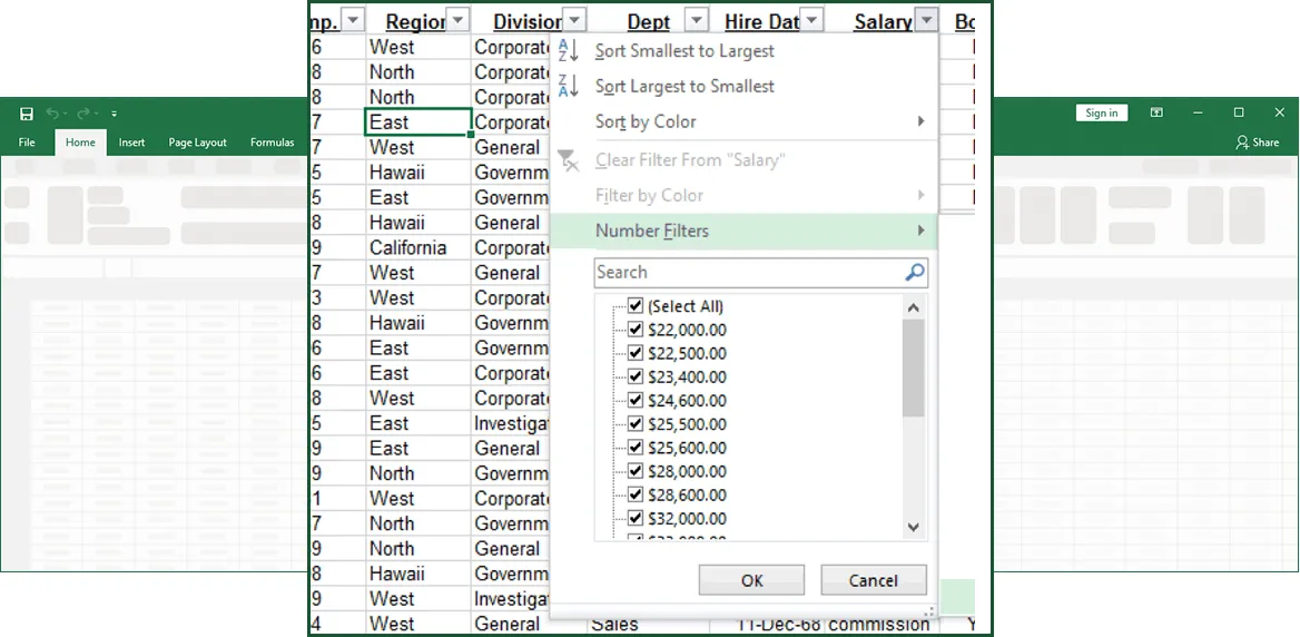
Figure 1-15A: Naviating to the Custom Auto Filter Dialog Box
Exercise
In the following exercise, you will customize AutoFilter criteria.
- Open the Fairfield Group workbook, and, if necessary, select the Canadian Operations worksheet.
- Select a cell in the list.
- In the Sort and Filter group on the Data tab, click the Filter button. [The AutoFilter drop-down arrows appear].
- From the Salary AutoFilter drop-down list, select (Number Filters...). [Another drop-down menu appears with number Filters options].
- In the next drop-down menu, select Custom Filter. [The Custom AutoFilter dialog box appears].
- In the Show rows where area, from the first comparison operator drop-down list, select is greater than or equal to.
- In the adjacent value drop-down combo box, type 40000.
- Choose OK. [Only the records in which the salary Is greater than or equal to 40,000 are displayed. The Salary AutoFilter drop-down arrow becomes a filter symbol].
- From the Salary AutoFilter drop-down list, click to select (Select All) and click OK. [All records are visible, and the Salary AutoFilter black drop-down arrow is back (filter icon removed)].
- From the Dept AutoFilter drop-down list, navigate to Custom Filter (note - text filter). [The Custom AutoFilter dialog box appears].
- In the first comparison operator drop-down list box, make sure equals is selected.
- From the adjacent value drop-down list, select Investigation.
- Select the Or option button.
- From the second comparison operator drop-down list, select equals.
- From the adjacent value drop-down list, select Marketing, and then choose OK. [Only the records for employees in the Investigation or Marketing department are displayed].
- From the Salary AutoFilter drop-down list, navigate to Custom Filter. [The Custom AutoFilter dialog box appears].
- From the first comparison operator drop-down list, select is greater than or equal to.
- In the adjacent value drop-down combo box, type 40000.
- Choose OK. [Only the records for employees in the Investigation or Marketing department with salaries greater than or equal to $40,000 are displayed, as shown in Figure 1-15B].
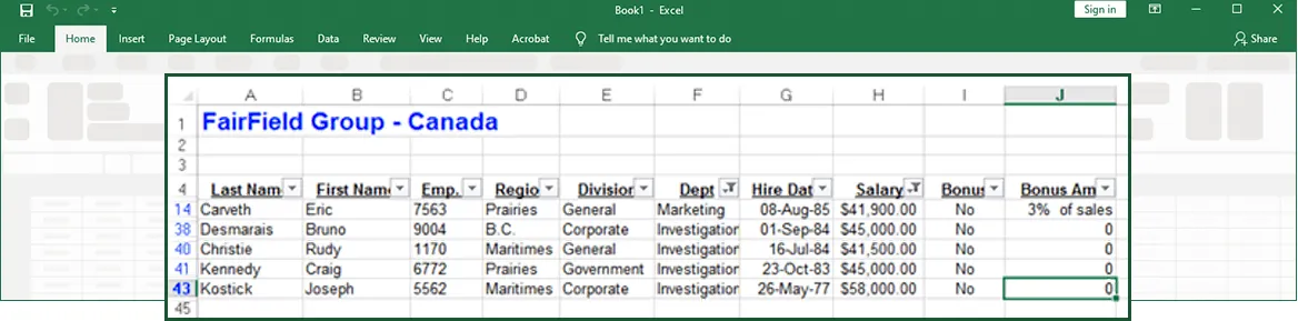
Figure 1-15B: The Filtered List (note filter icons next to the column labels on which the data is filtered)
Using the Top 10 Feature
Another option available from each AutoFilter drop-down list is the Top 10 feature. When you filter a list using the Top 10 feature, only the top number or the top percent of records remain. You can also filter to display the bottom number or the bottom percent of records. For example, if you want to list the top wage earners in the company, you can filter the Salary column to display only those records with the top ten salaries. If you filter for the top ten percent of wage earners, however, your list would include only those personnel whose salaries together equaled ten percent of the total.
Although called Top 10, you can filter for any number or percentage of items you desire. You make your selections for this feature using the Top Ten AutoFilter dialog box, shown in Figure 1-16.
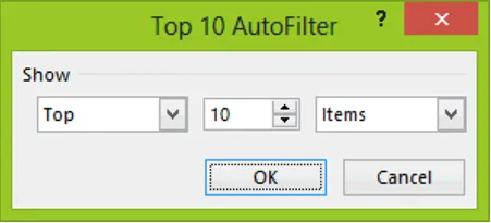
Figure 1-16: The Top 10 AutoFilter Dialog Box
Method
To use the Top 10 feature:
- If necessary, activate AutoFilter for the desired list.
- In the column with which you want to filter the data, from the AutoFilter drop-down list, select (Number Filters...). In the next drop-down menu, select (Top 10...).
- In the Top 10 AutoFilter dialog box, from the first drop-down list, select Top or Bottom.
- In the spin box, enter or select the desired number.
- From the second drop-down list, select Items or Percent.
- Choose OK.
Exercise
In the following exercise, you will use the Top 10 feature.
- Click a cell in the list.
- In the Sort and Filter group on the Data tab, click the Clear button. [The full list of data records is displayed].
- From the Salary AutoFilter select (Number Filters...), then in the next drop-down list, select (Top 10...). [The Top 10 AutoFilter dialog box appears].
- Make sure the following appear in the first drop-down list box, the spin box, and the second drop-down list box: Top 10 Items
- Choose OK. [Only the records of employees with the top ten salaries are visible].
- Display the full list.
- From the Salary AutoFilter drop-down list, select (Top 10...). [The Top 10 AutoFilter dialog box appears].
- Select the following in order in the first drop‑down list box, the spin box, and the second drop-down list box: Bottom 15 Percent
- Choose OK. [Only the records of employees whose salaries make up the bottom 15 percent are visible].
- Display the full list.
- Using the Top 10 AutoFilter feature, filter the list for the top 15 salaries. [Only the records of employees with the top fifteen salaries are visible].
Performing an Advanced Filter
You use the Advanced Filter command when you need to set more than two criteria or when you need to use a formula for computed criteria. You must create a criteria range before you can use the Advanced Filter command.
A criteria range is a range of cells that Excel uses to filter a list. The criteria range can be located anywhere on the worksheet outside of the list, and must contain some or all of the list’s field names and the desired criteria in the rows below them. The criteria range may span several rows, depending on compound criteria requirements. For example, to find records that meet criteria A and criteria B, enter the criteria in one row. To find records that meet criteria A or criteria B, enter the criteria in separate rows.
You enter the list range and the criteria range in the Advanced Filter dialog box, shown in Figure 1-17. A sample criteria range is shown in Figure 1-18.
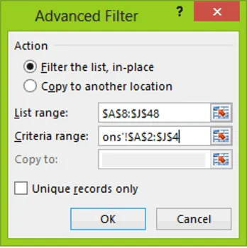
Figure 1-17: The Advanced Filter Dialog Box
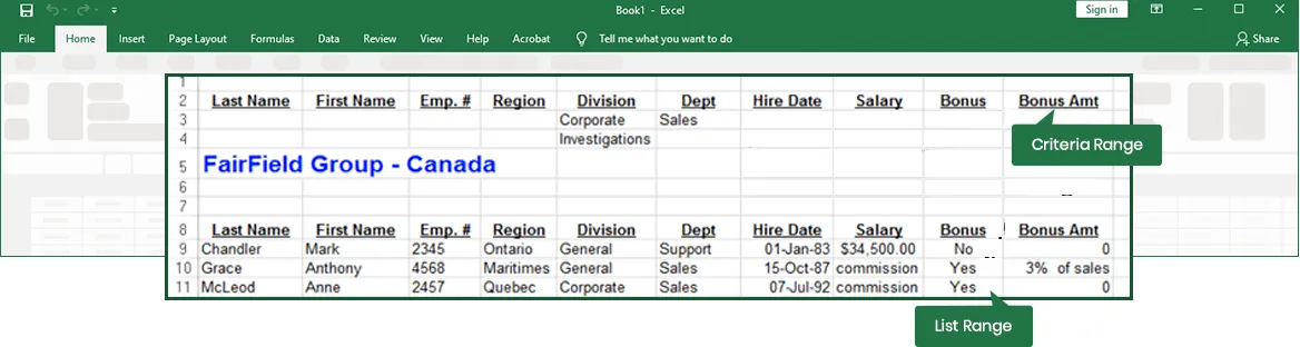
Figure 1-18: A Sample Criteria Range
Method
To perform an advanced filter:
- Copy the column headings you want to use for the criteria to an empty range on the worksheet.
- Below the appropriate copied column headings, enter the criteria.
- Select a cell in the list.
- In the Sort and Filter group on the Data tab, click the Filter button.
- In the Sort and Filter group on the Data tab, click the Advanced Filter button.
- In the Advanced Filter dialog box, in the Action area, select the Filter the list, in-place option button.
- In the List range text box, enter the desired list range.
- In the Criteria range text box, enter the range that includes the copied column headings and the criteria.
- Choose OK.
Exercise
In the following exercise, you will perform an advanced filter.
- Select the American Operations worksheet.
- Select the range A8:J8.
- Copy the range to A3:J3.
- In cell E4, enter Corporate. [The first criterion is set].
- In cell E5, enter Investigations. [The second criterion is set].
- In cell F4, enter Sales. [The third criterion is set].
- Select any cell in the list.
- In the Sort and Filter group on the Data tab, click the Filter button. [The Filter submenu arrows appear in headings].
- In the Sort and Filter group on the Data tab, click the Advanced Filter button. [The list is selected, and the Advanced Filter dialog box appears].
- In the Action area, make sure the Filter the list, in-place option button is selected.
- In the List range text box, make sure $A$8:$J$48 is displayed.
- In the Criteria range text box, type A3:J5.
- Choose OK. [Only the records of employees in the Sales department and in the Corporate or Investigations division are visible].
- Display the full list.
Copying Filtered Data to Another Location
When you filter data, Excel displays only those records that meet the filter criteria, and hides the records that do not meet the filter criteria. When performing an advanced filter, you can also copy your filtered data to another location on your worksheet, to let you compare your filtered list to your complete list.
To copy all the filtered data to another location, you click the Copy to text box, and then enter the upper left cell of the range to which you want to copy the filtered list. If the location to which you choose to copy the data contains any data, you will get an error message.
Method
To copy filtered data to another location:
- Create the advanced filter criteria range.
- Select a cell in the list.
- From the Data menu, choose Filter.
- From the Filter submenu, choose Advanced Filter.
- In the Advanced Filter dialog box, in the Action area, select the Copy to another location option button.
- In the List range text box, enter the desired list range.
- In the Criteria range text box, enter the range that includes the copied column headings and the criteria.
- In the Copy to text box, enter the upper left cell of the range to which to copy the filtered list.
- Choose OK.
Exercise
In the following exercise, you will copy filtered data to another location.
- Make sure the American Operation worksheet is active.
- In cell E4, enter Government. [The first criterion is set].
- In cell H4, enter >50000. [The second criterion is set].
- Delete the data in cells E5 and F4.
- Select a cell in the list.
- In the Sort and Filter group on the Data tab, click the Filter button. [The Filter submenu appears].
- In the Sort and Filter group on the Data tab, click the Advanced Filter button. [The Advanced Filter dialog box appears].
- In the Action area, select the Copy to another location option button.
- In the List range text box, make sure the range $A$8:$J$48 is displayed.
- In the Criteria range text box, change the existing range to $A$3:$J$4.
- In the Copy to text box, enter A50.
- Choose OK. [A copy of the filtered data appears below the list].
- Scroll to the bottom of the list to view the data. [Only one employee is listed].
- Save the workbook.