Customize Workbooks
In this article, will delve a little deeper into how to customize workbooks in Microsoft Excel.
For class based Microsoft Excel training in Los Angeles call us on 888.815.0604.
Your workbooks can be customized in a number of different ways. Over the course of this topic, we will focus on customization through the addition of comments, hyperlinks, watermarks, and background pictures.
Topic Objectives
In this topic, you will learn:
- About comments
- About hyperlinks
- About watermarks
Comments
Notes can be added to any worksheet by adding comments. Typically they are used to add additional context to items within a worksheet to help guide other users, but they can be used to add notes about any topic.
To add a comment, first select the cell that you would like the comment to be added to. Next, click Review → New Comment:
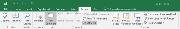
This action will create a new comment and a red comment indicator will appear in the upper right-hand corner of the currently selected cell. The comment will be labeled with the current user’s name, but this can be changed by replacing that text as needed. To add text to the comment, type inside the provided text area:
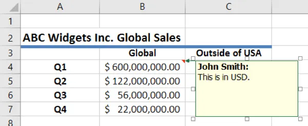
Once you are done, click anywhere outside of the comment text area to hide it; however, the red comment indicator will remain visible:
To view the comment again, click to select the cell in question or simply hover your cursor over it. To delete a comment, click to select the cell in which the comment has been placed and click Review → Delete.
Hyperlinks
Hyperlinks are a mainstay in the computing world. They enable you to navigate around your computer, browse the Internet, and jump to different cells within the same workbook. Excel lets you use this handy feature for breaking up long workbooks, pointing people to a web page, providing contact information, and much more.
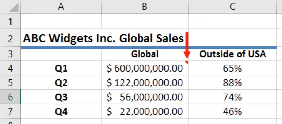
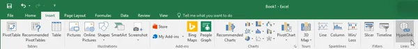
To create a hyperlink, first click to select the cell where you want the hyperlink to be created. Next, click Insert → Hyperlink:
This action will display the Insert Hyperlink dialog box.
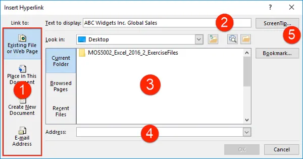
The left-hand side of the dialog allows you to choose the type of link (1) that you want to create. By default, the “Existing File or Web Page” option will be selected. (It will likely be the type of link you use most often.)
With this option, you will see the settings shown above. At the top of the dialog, you can set the text to display (2). This is the text that will turn blue and will contain the actual link. (By default, any text in the cell that you selected will appear in this field, but you can modify it if you wish.)
Below this field, you can choose the file (3) or website (4) that you want to link to. You can also set up a ScreenTip (5) for the link.
When you are ready, click OK to save your changes, or click Cancel to discard them. Note that the OK button will not be active until both the “Text to display” and Address fields are filled in.
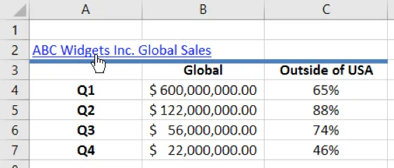
Once the hyperlink has been inserted, you will see that it appear blue and underlined. Clicking on the link will open it, but clicking and holding on the link will select the cell that contains it:
To remove a link, right-click the hyperlink in question and then click Remove Hyperlink in the context menu.
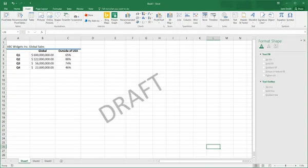
Watermarks
While Excel 2016 does not include a direct way to create watermarks, you can add them using WordArt. To do this, first insert WordArt by clicking Insert → WordArt → [WordArt Style]:

Next, type the text that you would like to make up the watermark and rotate it if needed:
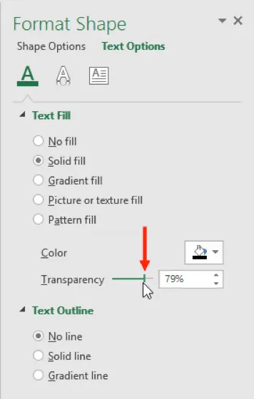
The watermark will now be ready and you can reposition it as needed: