Using the PMT Function
In this article, we will take a look into how to use the PMT Function in Microsoft Excel.
For instructor-led Microsoft Excel training in Los Angeles call us on 888.815.0604..
The PMT (payment) function is a financial function that is used to calculate loan payments based upon a constant interest rate. For example, if you take a loan of $10,000 at 6% annual interest over 4 years, you can use the PMT function to calculate what the monthly payment on the loan will be.
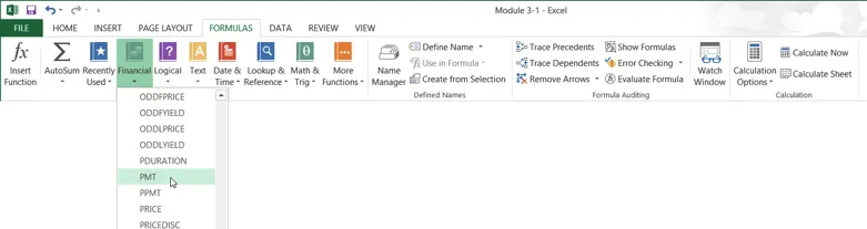
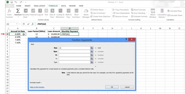
To use this function, first select the cell in which you want the results to be displayed. For this example, click cell D2. Next, click Formulas → Financial → PMT:
This action will open the Function Arguments dialog for the PMT function:
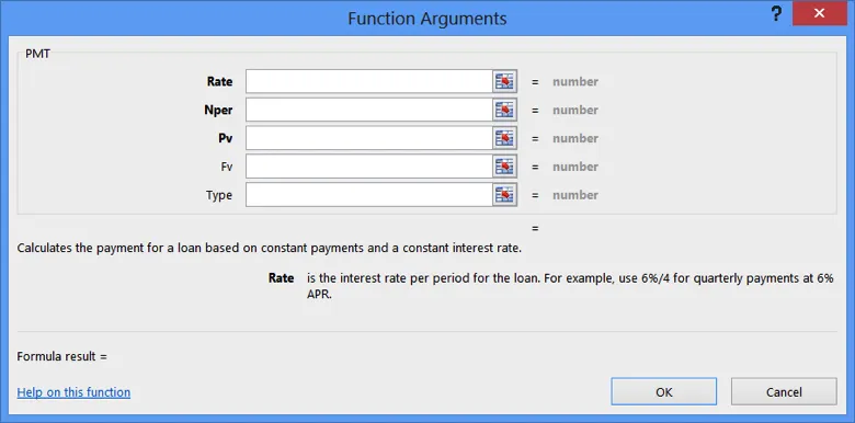
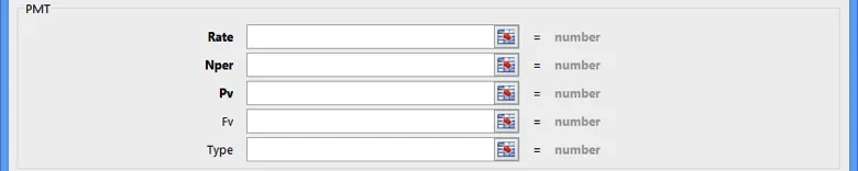
The top portion of the dialog contains a number of arguments for this function. Arguments that appear bold are required in order for the function to operate. Arguments not in bold are optional:
The Rate argument is the interest rate that will be used to calculate the payment. You have the option of inserting this number manually or selecting a cell in the current workbook that contains it.
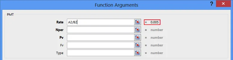
You need to account for the fact that the values in column A are annual interest rates, so you need to divide this data by 12. In the Rate argument field, type /12 after A2:
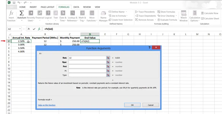
To start, click inside the Rate field. Next, with the Function Arguments dialog still open, click cell A2:
Now, type the divide operator (/) and then click cell B2:
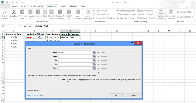
A2/B2 will now be displayed inside the Rate field. (This is used to calculate interest on a monthly basis.) The results of the information entered into this field will also be displayed:
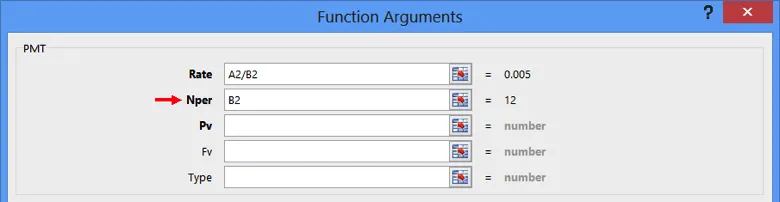
The Nper argument is the number of payment periods required for the loan. For this example, the worksheet already displays payment periods by the number of months in column B, so type B2 into this field:
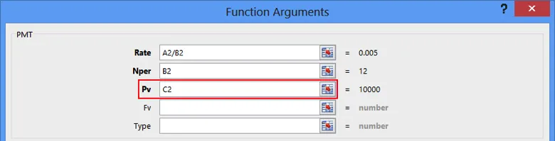
The Pv argument is the present value of the loan; in this case, the face value of the amount borrowed. Since loan amounts are listed in column C, type C2 into this field:
The remaining arguments listed in this dialog are optional.
- The Fv argument is used to specify an amount that is left outstanding after the loan payments are made for all payment periods. If you leave this option out, it will default to 0, meaning that the loan will be paid in full at the end of the payments.
- The Type argument will specify if the payment is made at the beginning or end of the payment period. If you enter an argument of 0, payments will be due at the end of the payment period. With an argument of 1, payments will be due at the beginning of the period. If you leave this argument out, it will default to 0.
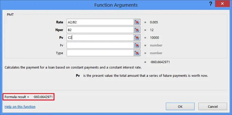
For this example, you can leave both of the optional arguments blank. The Function Arguments dialog will now look like the example below. As you can see, the formula result for this function is -860.66:
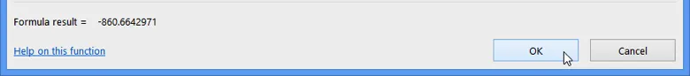
Click OK:
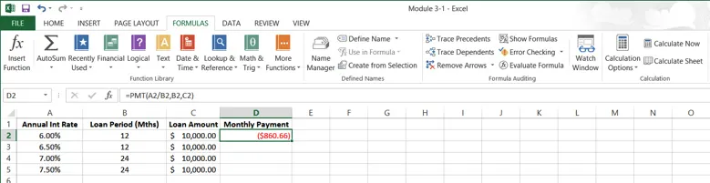
The results of the function will now be inserted into the cell you had previously selected. In this case, you can see that a $10,000 loan over the period of 12 months at an interest rate of 6.00% will require a monthly payment of $860.66:
Using AutoFill, apply this function to cells D3-D5:
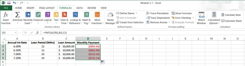
Keep in mind that when entering functions, you do not need to use the Function Arguments dialog. You can type this function directly into the formula bar using “PMT” as a prefix: